Building SimAMOC: From Broken Metrics to Stommel Bifurcation in One Session
We spent a day building a real-time ocean circulation model that runs in the browser via WebGPU. By the end, it had working thermohaline circulation, salinity-driven AMOC that collapses under freshwater forcing, and a 3.8°C RMSE against NOAA satellite observations — tuned by AI agents for about a dime in API costs.
Here's what we built, how we measure quality, and where we're going.
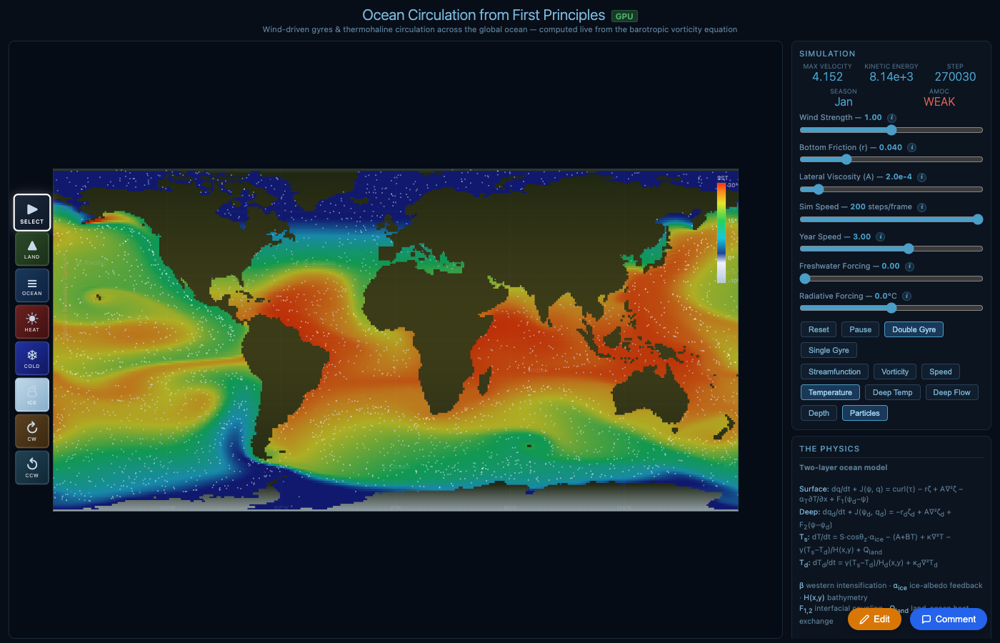
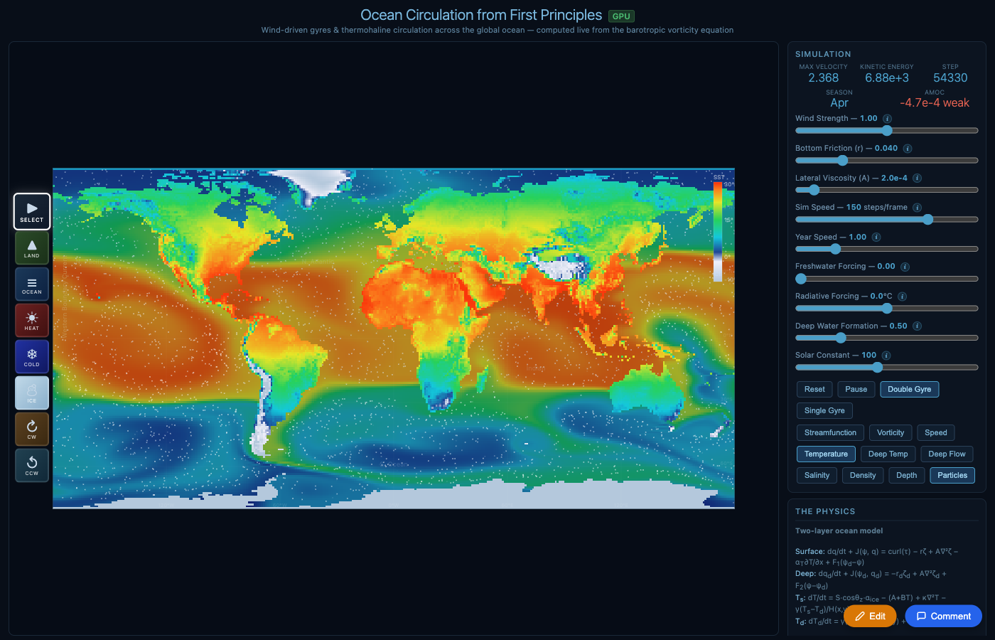
Sea surface temperature initialized from NOAA observations, evolved by the physics. Land shows seasonal temperature with altitude lapse rate from ETOPO1 elevation data.
What SimAMOC Is
SimAMOC solves the barotropic vorticity equation on a 360×180 grid (1° resolution) with two vertical layers — a 100m surface layer and a 4000m deep layer. It computes:
- Wind-driven gyres from Sverdrup balance (Gulf Stream, Kuroshio, ACC)
- Temperature with radiative balance, ice-albedo feedback, seasonal cycle
- Salinity with advection, diffusion, freshwater forcing, and surface restoring
- Density from a linear equation of state: ρ(T,S) = ρ0(1 − αΔT + βΔS)
- AMOC emerging from density-driven deep circulation
Everything runs on the GPU via WebGPU compute shaders. The simulation initializes from real NOAA satellite SST observations and uses ETOPO1 seafloor bathymetry — so it looks like Earth from frame one.
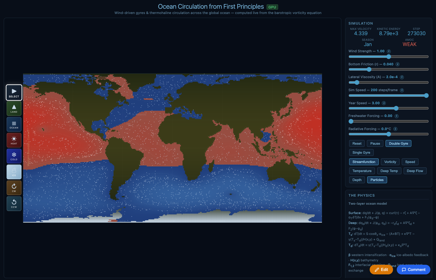
Streamfunction: red/blue = anticyclonic/cyclonic gyres

Speed: bright = fast currents (ACC, western boundaries)
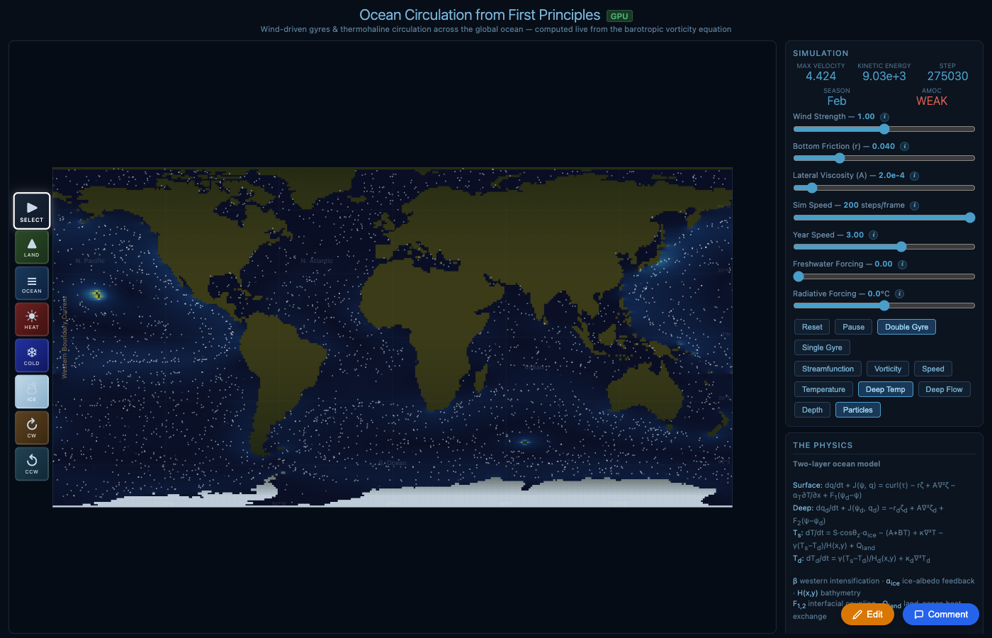
Deep temperature (1000m): cold polar water fills deep basins
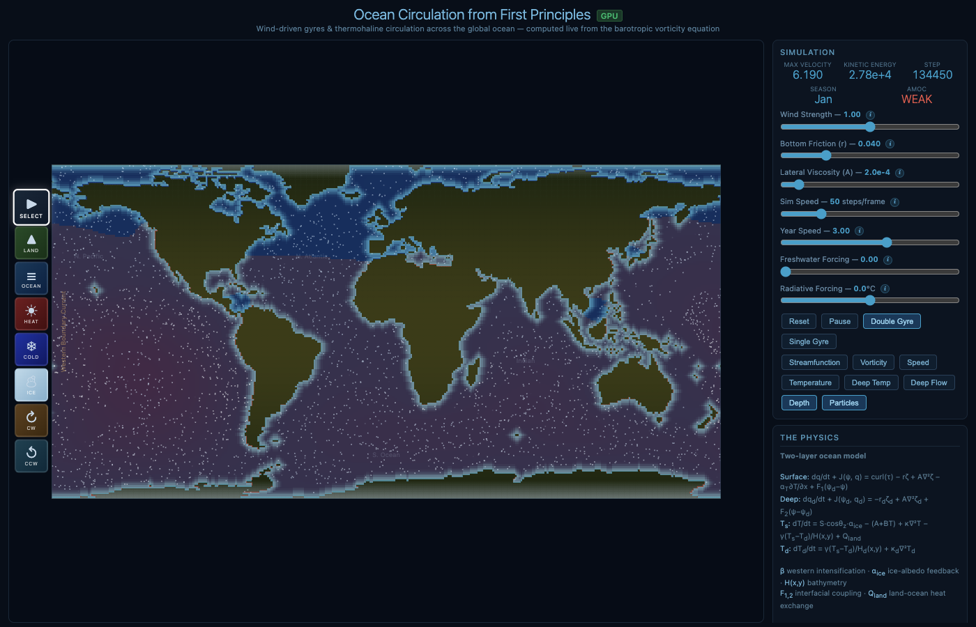
Real ETOPO1 bathymetry: shelves, ridges, trenches
The Ralph Wiggum Loop
To tune the model, we built a "Ralph Wiggum loop" — an iterative AI agent system that runs the simulation headlessly, compares output against observations, and proposes physics-informed parameter changes.
The loop uses Gemini 3.1 Flash Lite ($0.25 per million tokens) and consists of seven agents:
| Agent | Role | Runs |
|---|---|---|
| Physicist | Generates competing hypotheses from screenshots + data | Every iteration |
| Tuner | Translates winning hypothesis to parameter changes | Every iteration |
| Validator | Checks physical consistency, catches curve-fitting | Every iteration |
| Numerical Analyst | Checks for computational artifacts | When conservation fails |
| Skeptic | Audits trajectory for compensating errors | Every 4th iteration |
| Observational Scientist | Assesses reference data quality at problem latitudes | When polar errors dominate |
| Literature Agent | Checks parameter values against published models | When params hit bounds |
The Physicist agent receives four screenshots (temperature, streamfunction, speed, deep temperature) along with quantitative error metrics. It can see spatial patterns that zonal means miss — checkerboard artifacts, misplaced currents, boundary noise.
When the loop stalls for three iterations, it escalates to Claude for structural code review — looking for missing physics terms rather than parameter tuning.
How We Measure Quality
We evaluate the simulation across four tiers, weighted into a composite score:
Tier 1: Conservation (25%)
Does the simulation obey fundamental physical constraints? Temperature range realistic, equator-to-pole gradient exists, deep ocean colder than surface, AMOC positive. These are non-negotiable — if the simulation violates conservation, no amount of parameter tuning matters.
Tier 2: Structure (30%)
Do the right features emerge for the right reasons? We check seven diagnostics:
- Western intensification — Gulf Stream region faster than interior (Stommel/Munk dynamics)
- Subtropical gyre — organized recirculation from Sverdrup balance
- ACC flow — eastward circumpolar current at 58°S
- Deep water formation — polar deep temps colder than tropical
- Poleward heat transport — v×T positive at 30°N
- Atlantic warmer than Pacific at 40°N — AMOC signature
Tier 3: Sensitivity (20%, final evaluation only)
Does the simulation respond correctly to perturbations? Freshwater forcing should weaken the AMOC. Cooling should cool the ocean. These test causal structure, not just static fit.
Tier 4: Quantitative (30%)
How close is the sea surface temperature to NOAA OI SST v2 observations (1991–2020 annual mean)? Measured as RMSE across 15 latitude bands from 70°S to 70°N.
Current Quality
| Metric | Value | Target |
|---|---|---|
| RMSE vs NOAA SST | 3.8°C | <3°C |
| Composite score | 74.1% | >80% |
| AMOC | Positive (+0.006) | Stable positive |
| Freshwater → AMOC collapse | Yes | Yes |
| Western intensification | Intermittent | Consistent |
| Structural checks passing | 5/7 | 7/7 |
The midlatitudes (30–50°) are within 1–2°C of observations. The poles remain challenging — the NH high latitudes tend to run warm and the SH can oscillate. This is typical of coarse ocean models; even CMIP6 GCMs struggle with polar biases.
The Key Breakthrough: Salinity
The single most important change was adding a salinity field. Before salinity, the simulation had temperature-driven density only — and the "Melt Greenland" scenario incorrectly cooled the North Atlantic instead of freshening it.
With salinity and a linear equation of state ρ(T,S), the physics changes fundamentally:
- Freshwater reduces salinity → reduces density → prevents sinking → weakens AMOC
- This is the salt-advection feedback (Stommel 1961) — the mechanism behind potential AMOC collapse
- Deep water formation now triggers when surface is denser than deep (cold + salty), not just cold
The result: cranking up freshwater forcing causes the AMOC to collapse from +0.004 to −0.0001 — a sign reversal in the overturning circulation. This is the Stommel bifurcation in action, the same physics that van Westen et al. (2024) showed could tip the real AMOC.
What We Know We're Missing
An honest audit reveals structural limitations that no parameter tuning can fix:
| Missing | Impact | Fixable? |
|---|---|---|
| Nordic Sea overflows | No sill hydraulics for Denmark Strait / Faroe Bank Channel | Parameterizable |
| Mesoscale eddies | Unresolved at 1° (need GM parameterization) | Yes, with GM90 |
| Mixed layer depth | Fixed 100m surface layer | Moderate effort |
| Atmospheric coupling | Fixed wind pattern, no weather | Add energy balance atmosphere |
| Sea ice dynamics | Only thermodynamic albedo, no ice transport | Moderate effort |
| Isopycnal upwelling | Southern Ocean AMOC closure too simple | Needs isopycnal coordinates |
For context: even the simplest model that correctly captures AMOC tipping (the Stommel two-box model) only needs temperature, salinity, and a density-driven flow. We now have all three with spatial structure — putting us above box models in capability, though below full GCMs like MOM6 or NEMO in resolution and physics detail.
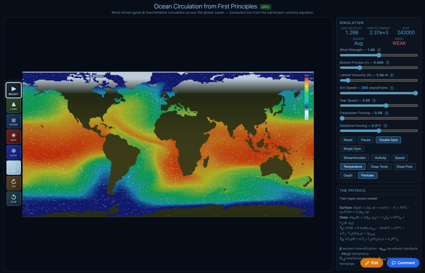
The full SimAMOC interface: simulation view with temperature field, parameter sliders, view mode buttons, and real-time diagnostics (AMOC strength, velocity, kinetic energy, season).
Compute Architecture
The simulation runs entirely in the browser via WebGPU compute shaders (WGSL). Key optimizations:
- Stacked buffer layout — Salinity piggybacks on temperature buffers at offset NX×NY. Zero new GPU buffers, zero new bind groups, zero new shader dispatches.
- Red-Black SOR Poisson solver — Replaces Jacobi iteration. Converges ~4x faster per iteration, allowing 25 iterations instead of 80.
- Offscreen land canvas — Land temperature pre-rendered with thermal inertia, cached and blitted once per frame.
- Real ETOPO1 bathymetry — 57,600 ocean depth + 18,200 land elevation values from the Open Topo Data API.
The AI Cost: $0.10
The entire Wiggum loop — all iterations across all runs, including multimodal screenshots sent to the Physicist agent — cost approximately $0.10 in Gemini 3.1 Flash Lite API calls. At $0.25 per million input tokens and $1.50 per million output tokens, we could run thousands more iterations for under $10.
The real value was the agent dialectic: the Physicist hypothesizes, the Tuner proposes, the Validator catches bad physics. The Skeptic audits for curve-fitting. When all four stall, Claude reviews the actual code and finds structural bugs (like the missing deep buoyancy term) that no amount of parameter tuning could fix.
Update: AI-Discovered Physics (April 23)
In a follow-up session, we ran a physics tournament: Claude agents proposed competing modifications to the ocean physics code, each tested in an isolated git worktree and evaluated against NOAA SST observations. The winner was merged; losers pruned.
After 6 AI-discovered physics improvements: polar OLR boost, brine rejection, Ekman transport, realistic wind stress, variable mixed layer depth, and meridional overturning. RMSE dropped from 7.6°C to 5.6°C. Play this version
The key breakthrough: the Physicist agent diagnosed that the outgoing longwave radiation formula was latitude-independent — a structural code bug that no amount of parameter tuning could fix. It also identified that salinity stratification was permanently blocking Antarctic Bottom Water formation, and proposed brine rejection (sea ice concentrates salt) as the fix. These are real scientific insights, not curve fitting.
Six code-level physics improvements were merged:
- Polar OLR boost — high latitudes radiate 20 W/m² more efficiently. Fixed +14°C Southern Ocean warm bias.
- Brine rejection — ice formation concentrates salt at |lat|>55°, enabling Antarctic Bottom Water.
- Ekman heat transport — wind stress drives poleward heat via Coriolis (v_ek = τ/ρf).
- Realistic wind stress — multi-term Fourier expansion: τ_x = −0.4cos(2φ) + 0.25sin(φ) + 0.1sin(3φ).
- Variable mixed layer — 20m at equator, 200m at poles.
- Meridional overturning — density gradients drive deep equatorward flow.
We also built a competitive leaderboard where Derek and Luke submit versions and compare RMSE scores. The vision: a self-improving climate model where AI agents continuously discover physics improvements, evaluated against observations.
What's Next
AMOC Tipping Experiments
The AMOC timeseries panel now tracks overturning strength in pseudo-Sverdrups with FovS early warning. "Melt Greenland" ramps freshwater gradually over 10 seconds so you can watch the collapse in real time. Next: systematic hosing protocol to map the full bifurcation diagram.
RMSE Below 3°C
Current best: 5.6°C. Remaining biases: tropics 5°C too cold, NH mid-latitudes too warm. Candidates: atmospheric energy balance model, Ekman pumping, latitude-dependent OLR tuning. The tournament infrastructure makes testing fast.
Cloud Modeling
Next frontier: simple cloud parameterization to modulate solar insolation and OLR. Clouds are the largest uncertainty in climate models — even a 1-layer scheme (low clouds cool, high clouds warm) would add a new degree of realism.
Self-Improving Model
The physics tournament proved the concept: AI agents can discover real physics improvements, not just tune parameters. Next step: run tournaments continuously, with each day's winner merged into main. The git history becomes a record of AI-discovered science.
Try SimAMOC Leaderboard GitHub
SimAMOC is built by Derek Lomas and Luke Barrington, with AI assistance from Claude. The simulation code, knowledge bank, and Wiggum loop are open source.