Real-time ocean circulation in the browser

An ocean model that
improves its own physics

The Atlantic meridional overturning circulation (AMOC) carries warm water north, keeping Europe 5-10°C warmer than it would otherwise be. It may be approaching a tipping point. SimAMOC simulates this system from first principles in the browser — and uses AI agents to discover and fix its own physics errors.

3.3°C
Best RMSE vs NOAA SST
5,249
Lines of simulation code
$0.10
Total AI tuning cost
20+
Observational datasets
60fps
Real-time in browser
Vision

Three layers of self-improvement

Climate model development takes years of PhD-level hand-tuning. We demonstrated in one session that AI agents can diagnose structural physics bugs, propose code fixes, and drop RMSE 37% — with zero human physics input.

Layer 1 — Built

Parameter Optimization

3-agent dialectic: Physicist diagnoses errors from screenshots, Tuner proposes parameter changes, Validator catches compensating errors. 13 tunable parameters, 4-tier evaluation.

RMSE 7.6 -> 4.7 in 10 iterations
Layer 2 — Built

Physics Code Mutation

Agents propose modifications to WGSL shaders and JS physics code. Each proposal runs in an isolated git worktree, evaluated against observations. Winners get merged.

Polar OLR, brine rejection discovered
Layer 3 — Future

Differentiable Physics

Port to JAX/WebGPU autodiff. Compute gradients of RMSE with respect to all parameters simultaneously. Combine gradient-based optimization with agent-based structural search.

Target: continuous improvement loop

What makes this different

Most ML-for-climate work builds emulators (faster but no new physics) or learns parameterizations from high-res simulations. We're doing neither. We're using AI to discover physics — to find missing equation terms, implement them in code, and validate against satellite observations. The git history becomes a record of scientific discoveries, each with a hypothesis, implementation, and observational validation.

Architecture

Browser-native ocean model

8 JavaScript modules sharing global scope, running physics on the GPU via WebGPU compute shaders with CPU fallback. Zero build step — just serve HTML.

model.js

Physics engine. All state arrays, ~50 parameters, 5 WGSL compute shader strings, CPU fallback solver, observational data loading. Zero DOM dependencies.

1,985 lines

gpu-solver.js

WebGPU compute pipeline. Buffer allocation, shader compilation, dispatch batching, CPU readback. FFT Poisson solver for exact streamfunction inversion.

881 lines

renderer.js

14 view modes, colormaps, GPU render pipeline, land elevation rendering with ETOPO1 bathymetry, particle overlays, diagnostic charts.

1,267 lines

main.js

Main loop orchestrator. GPU tick, atmosphere sub-stepping between readbacks, cloud field updates, and the window.lab API for automation.

265 lines

ui.js

Slider bindings for 9 physics parameters, 7 paint brush modes (SimEarth-style), and 6 paleoclimate scenarios (Drake Passage, Panama, Ice Age).

127 lines

overlay.js

Mobile-first drawer UI. Reparents controls into slide-out drawers, swipe gestures, speed presets (1x / 3x / 10x / MAX).

70 lines

Lab API

window.lab exposes the simulation to automation scripts via Playwright — the bridge between the browser and all external tooling.

lab.step(n)          // advance n timesteps
lab.diagnostics()    // extract SST, salinity, AMOC, zonal profiles
lab.getParams()      // read all parameters
lab.setParams({})    // inject parameter changes
lab.sweep()          // parameter sweep with scoring
lab.scenario(name)   // trigger paleoclimate scenario
lab.fields()         // extract raw field arrays
lab.reset()          // reinitialize from observations

Execution paths

ComponentGPU PathCPU Fallback
VorticityWGSL computeJS loops
Poisson solverFFT (exact)SOR (iterative)
TemperatureWGSL computeJS loops
AtmosphereCPU (between readbacks)CPU (every step)
RenderingWebGPU fragment + 2D overlay2D canvas only

Grid

512 x 160 cells at ~0.7° resolution. Latitude -79.5° to +79.5° (excludes polar ice caps). Periodic in longitude.

All derivatives include cos(lat) metric correction. Coriolis parameter clamped near equator (|lat| < 5°) to avoid singularities.

Why this size? All climate data products (WOA23, NOAA SST, NCEP wind, MODIS clouds) are distributed at 1° on this grid. 81,920 cells total — fast enough for real-time on mobile GPUs.

Physics

What the ocean does, and how we model it

One equation produces all major ocean currents. Wind stress curl drives the gyres. The beta effect creates western intensification. Temperature and salinity gradients drive the overturning circulation.

Surface vorticity — wind-driven circulation + buoyancy
dq/dt + J(psi, q) = windCurl - r*zeta + A*laplacian(zeta) - alpha_T*dRho/dx + F*(psiDeep - psi)
Surface temperature — radiation + advection + mixing
dT/dt = -J(psi,T) + S*cosZ*iceAlbedo*cloudAlbedo - (A_olr + B_olr*T)*(1 - cloudGH) + kappa*lap(T) - gamma*(T-Td)/H
Density — linear equation of state
rho = rho_0 * (1 - alpha*dT + beta*dS)

Feedback loops

The model's behavior emerges from coupled feedbacks, not individual terms.

What the model can represent

  • Wind-driven subtropical & subpolar gyres
  • Western boundary currents (Gulf Stream, Kuroshio)
  • Antarctic Circumpolar Current
  • AMOC and freshwater-driven collapse
  • Seasonal cycle with ice-albedo feedback
  • Cloud radiative effects (7 regimes)
  • Paleoclimate scenarios

What it cannot

  • Mesoscale eddies (need ~0.1°)
  • Gulf Stream separation at Cape Hatteras
  • Sea ice dynamics (only thermodynamic)
  • Nordic Sea overflows
  • Realistic mixed layer dynamics
  • Tidal mixing
  • Diurnal cycle
Visualization

14 ways to see the ocean

Every field the model computes can be viewed in real-time. Click any image to launch the simulation.

Data Pipeline

Grounded in observations

The model loads 10 observational datasets at runtime — SST, deep temperature, bathymetry, salinity, wind stress, albedo, precipitation, and cloud data. It initializes from the real Earth, not a blank canvas.

DatasetSourceUsed forPeriod
Sea surface temperatureNOAA OI SST v2Init + RMSE scoring1991-2020
Deep temperature (1000m)WOA23Deep layer initializationClimatology
Bathymetry + land elevationETOPO1Depth field, terrain renderingStatic
Surface salinityWOA23Salinity restoring target1991-2020
Wind stress (tau_x, tau_y)NCEP ReanalysisWind curl + Ekman transport1991-2020
Surface albedoMODIS MCD43A3Land surface albedo2020-2023
PrecipitationGPM IMERGCloud parameterization2015-2023
Cloud fractionMODIS MOD08_M3Cloud model validation2020-2023
Cloud types (low/high)MODIS MOD08_M3Radiative effect calibration2020-2023
Land/ocean maskNatural Earth 110mDomain boundariesStatic

High-resolution data ready

20+ fields at 1024x512 resolution, fetched via Google Earth Engine. Includes monthly climatologies for wind stress and albedo. Waiting for the GPU FFT solver to support larger grids.

Time series available

RAPID AMOC (26.5°N), CO2 from Mauna Loa, GISTEMP, HadCRUT5, HadSST4, ocean heat content, Arctic/Antarctic sea ice extent. Available for driving scenarios and validation.

NOAA SST WOA23 ETOPO1 NCEP Wind MODIS Clouds GPM Precip
Google Earth Engine + WOA23 pipelines
10 JSON files at 360x160 model.js GPU shaders (WGSL) renderer.js Screen
window.lab API via Playwright
wiggum-loop.mjs tournament.mjs tune.mjs versions/ leaderboard
AI Self-Improvement

The Wiggum Loop

Named after the Ralph Wiggum pattern — AI agents iteratively diagnose what's wrong with the physics, propose fixes, and validate them. At ~$0.03 per run, we can afford thousands of iterations.

Core Agent

Physicist

Sees 4 screenshots + scorecard + zonal error profiles. Produces 2-3 ranked hypotheses about what's physically wrong.

Core Agent

Tuner

Translates the winning hypothesis into parameter changes. Max 3 parameters, max 30% step. Respects published physical bounds.

Core Agent

Validator

Checks physical consistency, catches compensating errors. Can reject proposals that improve one metric while degrading others.

Evaluation tiers

Not all metrics are equal. A model that fits SST perfectly but has wrong AMOC dynamics is worse than one with 1°C higher RMSE but correct tipping behavior.

T1: Conservation

Binary gate. Energy balance, temperature range, stratification, AMOC positive. Failing T1 caps the score.

T2: Structure

35% of score. Western intensification, gyre existence, ACC flow, deep water formation, poleward heat transport.

T3: Sensitivity

20% of score. Freshwater weakens AMOC, cooling cools ocean. Tests correct response to perturbations.

T4: Quantitative

35% of score. Zonal-mean SST RMSE vs NOAA observations. The hard number — currently 3.3°C.

On-demand specialists

Triggered by conditions, not every iteration:

  • Numerical Analyst — when T1 conservation fails (checks for computational artifacts)
  • Skeptic — every 4th iteration (audits for curve-fitting and parameter drift)
  • Literature Agent — when parameters hit bounds (checks published model values)
  • Claude — when stalled 3 iterations (structural code review)
Development

Built in five days

A collaboration between Luke Barrington (original physics engine + GPU compute) and Derek Lomas (salinity, AI loop, data pipeline, clouds, atmosphere, documentation).

Pre-session (Luke Barrington)
v1-v4: Barotropic vorticity + WebGPU
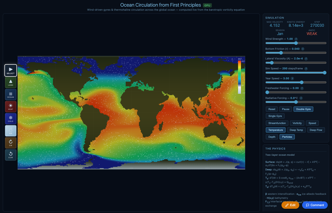
Wind-driven gyres, western boundary currents, ACC, temperature field. Paleoclimate scenarios, SimEarth-style paint tools, real coastline mask at 1°.
April 21 (Claude + Derek)
Wiggum loop + salinity + real bathymetry
3-agent AI tuning loop, full salinity field with density EOS, ETOPO1 bathymetry, SOR Poisson solver, observed SST initialization. AMOC goes positive for the first time. Freshwater collapses AMOC (Stommel bifurcation live).
RMSE: infinity -> 3.8°C
April 23 (Luke + Derek)
FFT Poisson + Ekman + variable MLD
cos(lat) metric correction, FFT Poisson solver (exact), Ekman heat transport from wind stress, variable mixed layer depth by latitude. AMOC timeseries panel with RAPID reference.
RMSE: 3.8 -> 3.3°C
April 24 (Claude + Derek)
Cloud model + atmosphere + wind stress
7-regime cloud parameterization, 1-layer atmospheric energy balance with two-way coupling, ERA5 wind stress, Southern Ocean cloud fix, MODIS cloud type validation data.
Physics: +clouds, +atmosphere, +moisture
April 25 (Claude + Derek)
Physics registry + system documentation
Complete inventory of every physical process with equations, data sources, status, and known gaps. Interaction map showing all feedback loops and parameter sensitivity chains.
PHYSICS_REGISTRY.md + SYSTEM.md
74%
Peak composite score
20
Versions submitted
2
Contributors competing
16
Knowledge bank files
Roadmap

What's next

Immediate

  • Fix GPU FFT Poisson solver (currently forced to CPU+FFT fallback)
  • Retune parameters with cloud model active (RMSE regressed from 3.3 to ~7.2°C)
  • Wire snow-albedo feedback (MODIS data downloaded, not yet used)
  • Upload airTemp to GPU for physically consistent atmosphere coupling

Short-term

  • Improve AMOC diagnostic (zonally-integrated transport, not point velocity)
  • AMOC hosing experiments with hysteresis testing
  • Support 1024x512 grid (high-res data pipeline already built)
  • Automated CI testing via GitHub Actions

Medium-term

  • GM-like eddy parameterization for 1° resolution
  • Multi-layer atmosphere with Hadley/Ferrel cells
  • Sea ice model (thickness, drift, brine rejection)
  • Validate against ECCO v4 state estimate

Vision

  • RMSE < 2°C (requires higher resolution + better physics)
  • Reproduce AMOC tipping with realistic freshwater timeline
  • Train neural network emulator for instant scenario exploration
  • Publish methodology paper on AI-assisted ocean model development